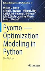
Rating: 8.2/10.
Book giving an overview of the Pyomo optimization framework, which doesn’t solve optimization problems itself but allows users to formulate them in a high-level, object-oriented format. Pyomo acts as an interface with solvers like CPLEX. The book talks about into numerous features of Pyomo but mostly stays clear of the solver algorithms’ internals, as well as the performance characteristics of the solvers—it focuses primarily on the Pyomo translation layer and discusses managing complex systems of constraints efficiently.
Chapter 1. Algebraic modeling languages (AML) allow for a high-level description of a problem, and Pyomo leverages Python’s object-oriented features instead of requiring a specialized language. In this setting, you can define model variables, objectives, and constraints directly in Python; the framework is extensible and supports a wide variety of mathematical models and solvers.
Chapter 2. Basics of optimization models. A decision variable, often the letter x, is the element we aim to solve for. Parameters (or data), are the values used to describe the specific instance of the problem. Every model must include an objective function and various constraints, which can be defined in numerous ways using Pyomo. In linear programming, both the objective function and the constraints must be linear in terms of the decision variable, although they can be nonlinear in non-decision parameters. Pyomo itself doesn’t solve the problem; instead, it passes the instance to a solver.
Chapter 3. Overview of Pyomo objects and formulating a warehouse location problem. Decision variables are created using the Var object and can have bounds, initial values, and domains, such as integer or non-negative. While constraints can be written one at a time, this approach can be tedious; alternatively, indexed constraints allow you to set many constraints at once using construction rules. For cases where one constraint or objective depends on multiple parameters, you can define them using list comprehension. For Set and Param, some functionalities can be replicated using Python types, but certain features are only available using these Pyomo objects, like if you want to solve the model multiple times with different inputs without needing to reconstruct the model.
Chapter 4. More detailed overview of each Pyomo component. Variables represent either a single value or an indexed set of values; the domain of the variable can be specified by a predefined virtual set, such as positive integers, or by a set of values that it can take. They can also have bounds specified by a tuple or you can set initial values. A variable can be fixed to a constant as well.
Objectives can be defined using either an expression or a Python function. While it’s possible to specify multiple objectives per index, this practice is uncommon. Constraints, on the other hand, are often indexed—there is typically one constraint for each combination of indices. They can also be defined by expressions, and you can choose to skip a rule for certain indices to indicate that there is no constraint for that specific combination of indices.
The Set object defines a collection of items, and beyond the Python set, you can define relationships between different sets, such as subsets, and validate their properties.
Parameter data is managed within the Param class, which simplifies the initialization of parameters with defaults and then setting some indexes. By default, parameters are converted to constants immediately, but if set to mutable, they are converted just before passing to the solver. When parameters are defined in a sparse representation with many defaults, they are stored in a sparse format but appear dense in their interfaces.
Finally, the Suffix component is used for bidirectional communication of data to and from the solver; they can be attached to any model component to set a suffix.
Chapter 5. The most basic script for optimization involves reading the data, defining the model, calling the solver, and printing the results. You can obtain specific information from the solver, such as the values of the objective function and each variable. The value function retrieves the numeric value for a variable or parameter; this is crucial because performing arithmetic operations on variables otherwise creates an expression. You can make various changes to a model without reconstructing it, such as disabling constraints, fixing a variable to a constant, so you can rerun the model.
A common workflow involves successively adding cuts to a model after each solution is generated to eliminate that solution and run the model again; this process finds multiple solutions. You iterate until all solutions are found, at which point the model becomes infeasible. The chapter provides an example of how to apply this technique to solve a Sudoku puzzle and find all possible solutions.
Chapter 6. You can pass additional options to a solver, such as the location of the log file, solution file, time limit, etc. Results are directly updated in the model, so the results object only contains supplementary information and not the solution itself.
Chapter 7 discusses nonlinear programming, where you’re not limited to just linear functions with Pyomo but can use operations like multiplication, exponentiation, trigonometry, and logarithms. However, you can’t use just any arbitrary function since they typically require an automated way to evaluate first or second derivatives. Unlike linear optimization, initialization tends to be more critical here, and finding a global optimum is generally less likely.
Some examples include: solving a nonlinear system that models the harvesting of deer and an SIR model for infectious diseases: this one is a least squares estimation problem of fitting the SIR model parameters optimally. The formulation introduces a variable epsilon, representing the residual and the objective is to minimize the sum of these residuals.
Chapter 8 introduces the block component, which is beneficial for organizing a model into a structured hierarchy rather than managing everything globally. While variables within blocks are accessible globally, best practice is to only refer to child blocks. Blocks can be initialized using rules akin to constraints, with the rule’s first argument being the block itself, not the entire model. This structure is particularly helpful for simplifying formulations, as generalizing a problem instance to solve several instances simultaneously often requires adding a new index. By using blocks, you can construct individual blocks as usual and then apply rules to link these blocks together.
Chapter 9: Performance. Various tools and utilities for timing and profiling to pinpoint slow parts of the program. The slowness could be due to either model translation time or solve time. While there’s not much that can be done to speed up the solver itself, there are numerous ways to enhance the efficiency of translating from Python to the solver’s language. One method is using LinearExpression to formulate constraints; it’s more low-level but faster.
Persistent solvers come into play when you’re solving the same model with minor variations repeatedly. However, they require extra work to keep in sync: eg, to remove constraints, you need to call the remove function instead of simply reassigning the variable. Sparse index sets prove useful when you would otherwise employ many Constraint.Skip statements for invalid index combinations.
Chapter 10. Abstract models build a general model without specific data, while concrete models create a model with actual data. The choice between the two comes down to preference, with concrete models often being easier for those familiar with Python, as they involve direct manipulation of Python data structures. On the other hand, abstract models are more similar to traditional AML workflows. In an abstract model, the script is concerned only with setting up the model structure. It uses Param to denote a placeholder for data and initializes it with dimensions rather than real data, which is provided later when the model is filled in prior to solving.
Solving abstract models typically uses the pyomo solve command. This command requires a Python script that initializes a model in a variable named “model,” with data specified in a Pyomo specific format similar to the AMPL format. You can define custom steps as part of the workflow with Python functions. These functions can serve as callbacks during the Pyomo solve process, for example, to output results in a custom format.
Chapter 11. Generalized Disjunctive Programming (GDP) is useful for formulating problems with multiple constraint groups where at least one group must be satisfied. This is modeled using the Disjunct component, similar to the Block component. For solving, it can be transformed into a MIP through the Big M or hull transformations. An example of a GDP is ensuring constraints are met while minimizing the number of non-zero inputs.
Chapter 12. Differential Algebraic Equations (DAEs) involve minimizing the value of a differential equation at a certain time point, given initial conditions. In Pyomo, DerivativeVar is used to represent differential equations, while fix is used for setting initial conditions. These equations are typically transformed using either finite difference methods, which discretize the problem, or collocation methods, utilizing polynomial approximations.
Chapter 13. Mathematical Programs with Equilibrium Constraints (MPEC) problems arise in systems that deal with equilibria and can be modeled using complementary expressions. They can then be automatically transformed into disjunctive programs.


