Rating: 8.3/10.
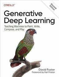
Generative Deep Learning: Teaching Machines to Paint, Write, Compose, and Play by David Foster
Book covering the fundamentals of all the major generative AI models, focusing on image generation such as VAE, GAN, diffusion models, etc. It presents relatively little math and uses Keras code to demonstrate how to train and run each of the models. The first half of the book presents all the major building blocks that are frequently used in generative AI; I like how it uses analogies to build intuition before diving into the details. The second half focuses more on specific tasks and the state-of-the-art models that are currently used to solve these tasks; the second part was relatively weaker, and a lot of random architectural details are thrown at you quickly. Some chapters were a bit strange, such as the music generation, which is generally not done this way. The reinforcement learning chapter picks an obscure world-based model, which was an odd choice for a first introduction to RL.
Chapter 1. Generative modeling aims to generate new samples that are similar to the training data, whereas discriminative models learn how to label data. Generally, this means learning the distribution from which the data is drawn and then, to sample, we can simply draw from the same distribution. A latent space is a lower dimension space that has higher level features, often we sample from this latent space and transform it back to the original space.
The general framework is that you find a set of maximum likelihood parameters, \theta, that most likely explains the data, X. Generally, the density function is intractable to calculate directly, so avoid modelling this explicitly (like GAN, which just learns to produce samples without any distribution), or model an approximate distribution that is more tractable.
Chapter 2: Basics of deep learning; components of NN; loss functions, optimizers, training and evaluation; building a CNN classifier for CIFAR10 using Keras.
Chapter 3. The autoencoder consists of two parts: the encoder encodes the input to a latent vector, and the decoder reproduces the original input using a reconstruction loss. The latent space groups similar items together, but many empty areas and different categories are spread out differently, making it difficult to sample from it.
The solution to this is the variational autoencoder (VAE). Here, instead of producing a vector, the encoder produces a mean and variance vector that represents a multi-dimensional normal distribution. This distribution is then randomly sampled before being fed into the decoder. The log of the variance is used so that the network can produce negative values (as the variance cannot otherwise be negative). The reparameterization trick adjusts the sampling operation by adding a standard normal random sample to it, allowing for backpropagation. A KL loss with a standard normal distribution is used to keep the model’s latent distributions close to the origin. The combined loss is the sum of the KL loss and the reconstruction loss. This way, the learned representation still groups similar samples together, but sampling from it more reliably produces valid images.
Chapter 4: Generative Adversarial Network (GAN) has a discriminator that predicts whether an image is real or generated, and a generator that takes a random vector and transforms it into an image. A major challenge in training a GAN arises when the discriminator is too strong, as the generator cannot improve if it can never fool the discriminator. Alternatively, if the discriminator is too weak, it can result in mode collapse, where the generator always produces a small set of similar images. Therefore, this model is relatively sensitive to hyperparameters.
The solution to this is the Wasserstein GAN (WGAN). Instead of using a discriminator, it uses a critic network to predict arbitrary positive and negative numbers, as opposed to just 0 and 1, and it aims to maximize the difference between real and generated images. One mathematical condition necessary for this to work is for the critic function to be 1-Lipschitz. This avoids any collapse of the loss function when the discriminator is too strong; in fact, the critic may be trained to be as strong as you like, and the loss surface for the generator will still remain informative.
The Lipschitz condition is typically enforced using a gradient penalty. This involves sampling a random selection of interpolated images between real and fake ones, taking the gradient of the critic network at that point, and then penalizing when the gradient is too high. A variant of WGAN is Conditional GAN (CGAN), which can generate different classes of images: during training, a label vector (one hot encoded) is appended to both the generator and critic, in order to control which class is generated.
Chapter 5. Autoregressive model generates a sequence one token at a time, example is training an LSTM on a recipes dataset. Extensions to LSTM include stacking and bidirectional methods. PixelCNN generates images autoregressively by predicting one pixel value at a time, assuming black and white, and 256 possible monochromatic values. This is done using a masked Conv 2D layer that only has access to previous pixels and a residual block at each layer. This process is very slow compared to GAN and VAEs because one pixel is generated at each step. One optimization method is to output a mixture distribution instead of 256 independent color values, and sample from it.
Chapter 6: Normalizing flow models learn a transformation from the original data distribution to a standard normal distribution that is invertible. This allows you to sample from a normal distribution and invert the process to generate new images, but means all network operations must be invertible; additionally, they must have a determinant that is easy to compute, as you need the determinant of the Jacobian to preserve the volume during the change of variable transformation and to remain a probability density function. RealNVP accomplishes this through a coupling layer, constructed with masking in a specific way, so that the transformation is a lower triangular matrix, so that the determinant is known and is also invertible. The model alternates stacking two types of coupling layers, allowing different halves of the vector to be transformed in different layers, and is trained to approximate the Gaussian distribution. More recent improvements of normalizing flow models include GLOW and FFJORD.
Chapter 7: Energy-Based Models (EBM) – the goal is to train a neural network to assign low values to real images and high values to generated images. Then, during inference, we take a random point and apply gradient descent (not on parameters, but on the image) to adjust it to a lower energy function value. Note that there is no decoder neural network involved at all. The principle of contrastive training is that real images should score lower than generated images; generated images are obtained by sampling a random point and applying the same sampling procedure a few times (process called Langevin dynamics sampling). Older EBM models include the Boltzmann machine and deep belief networks, but there is no efficient way to train them on high-dimensional data.
Chapter 8: Diffusion models learn to predict random noise into an image. The forward diffusion process starts with a clean image and progressively adds noise until it is completely random. The diffusion schedule controls the rate at which this happens, and the cosine schedule works better than the linear schedule as the noise ramps up more slowly. The model is trained to predict the noise that is added so that it can be iteratively undone; the U-Net architecture is used because the predicted noise is the same shape as the image. The architecture consists of several down blocks followed by up blocks with residual skip connections to cut across the unit from the down blocks directly to the corresponding up block. Note that the model is not aware of the diffusion schedule, so it predicts the total amount of noise and not one timestamp of noise (since it cannot know how much noise should be removed in one timestep). So at inference time we can use a different number of steps as during training because each step will partially subtract the predicted noise.
Chapter 9: covers the transformer architecture, including self-attention, causal masking, positional embeddings, and various types of transformers such as encoder-only and encoder-decoder, variants of the GPT models.
Chapter 10: Advanced GANs. ProGAN first trains the discriminator and generator on 4×4 down-sampled images and gradually scales it up to higher resolutions, each time it scales up, it adds a layer to both the generator and discriminator, but keeps the original path for some time for a transition period. During this period, the original path is gradually phased out. This strategy avoids the shock of adding a randomly initialized layer to the network. StyleGAN has a mapping network that produces a style vector, which is injected into the generator several times at different layers. It uses an adaptive instance normalization layer to ensure that the style information does not propagate to later layers. StyleGAN2 resolves some of the artifacts of the previous model and simplifies the progressive growing layer scheme and is SOTA on many face generation tasks.
SAGAN uses self-attention to improve the long-range dependency structure, and BigGAN is similar but larger. VQVAE learns a codebook of label-to-vector mapping (think of this as vocabulary), each image is decomposed into a grid, and each grid cell is represented by one label in the codebook. VQGAN is a modification to this – it’s useful to have a GAN discriminator as part of VAE because otherwise, the VAE tends to generate blurry images. Vision Transformer can also be incorporated into this architecture.
Chapter 11: Music Generation. In its simplest case is when the music is monophonic, it can be modeled as a sequence of notes and durations, a transformer, can be used to predict the next note and duration auto-regressively. However, the case for polyphonic music is more complicated, as many simpler representations cannot handle complicated rhythms and repeated notes. A more flexible representation is a stream of events, where each event can be a note turning on or off at a given timestep. MuseGAN is a paper published in 2017, uses a GAN to generate Bach chorales. It converts a chorale into an array of note values, one for each voice, and generates one bar at a time, treating it as an image generation problem. The generation process has four inputs: melody, chord, style, and groove, to allow for different control of style over the four voices.
Chapter 12: introduces world model for reinforcement learning. In the car racing environment, a VAE is first used to learn a latent representation of the world state, where data is collected from random rollouts. Then, a RNN is trained to predict the next state and reward of a given action. Finally, an evolutionary algorithm is used to learn a controller neural network (in this setup, there is no gradient to learn from). Essentially, the controller learns in the “dream” environment, modeled by the RNN, without ever encountering the real environment.
Chapter 13: Image generation from text models – DALLE 2 from OpenAI uses CLIP, a model that encodes text and vision into a common latent space and has strong discriminative power on many datasets. The prior model converts text embedding into image embedding, and for this piece, the diffusion model works better than autoregressive. The final decoder is a diffusion model conditioned on both text and image embedding, producing a 64×64 image. This image is then upsampled using another diffusion model. Technically, the prior model is not necessary in this architecture, but better results are achieved this way than just decoding from CLIP text encoding. The limitation is errors when multiple objects with different attributes get entangled, and the spelling is poor.
The Imagen model from Google is similar but uses the text encoder T5 instead of CLIP. Stable Diffusion is open source and one difference is that the diffusion operates on a latent space rather than images, with an auto encoder to handle encoding and decoding images from the latent space. The Flamingo model from DeepMind is multimodal and can handle a video as a sequence of images that is encoded into a latent vector to avoid long sequence computational complexity; it modifies the Chinchilla LM to be able to process images.
Chapter 14 – Conclusion. This chapter categorizes the history of generative AI into three eras. The first era is that of VAE and GANs, followed by the era of transformers, and then the current era of big models. Overview of all the major models at the time of the book’s publishing in early 2023, and thoughts on the future directions of generative AI.
